7.1 Sources of error when doing inference and generation with Inflationary Flows
Several previous lines of work (Gneiting & Raftery, 2012; Diebold & Mariano, 2012; Malinin & Gales, 2018; Yao et al., 2019; Urteaga et al., 2021) have focused on assessing how well model-predicted marginals \( p(\mathbf{x}) \) match real data (i.e., the predictive calibration case). Though we do compare our models’ predictive calibration performance against existing injective flow models (see Experiments on image benchmark datasets), here we are primarily focused on quantifying error in unconditional posterior inference. That is, we are interested in quantifying the mismatch between inferred posteriors \( q(\mathbf{z}|\mathbf{x}) \) and true posteriors \( p(\mathbf{z}|\mathbf{x}) \), especially in contexts where the true generative model is unknown and must be learned from data. This is by far the most common scenario in modern generative models like VAEs, flows, and GANs.
As with other implicit models, our inflationary flows provide a deterministic link between complex data and simplified distributions with tractable sampling properties. This mapping requires integrating the proposed general pfODE for a given choice of \( \mathbf{C}(t) \) and \( \mathbf{A}(t) \) and an estimate of the score function of the original data. As a result, sampling-based estimates of uncertainty are trivial to compute: given a prior \( \pi(\mathbf{x}) \) over the data (e.g., a Gaussian ball centered on a particular example \( \mathbf{x}_0 \)) , this can be transformed into an uncertainty on the dimension-reduced space by sampling \( { \mathbf{x}_j} \sim \pi(\mathbf{x}) \) and integrating the general pfODE forward to generate samples from \( \int p(\mathbf{x}_T|\mathbf{x}_0)\pi(\mathbf{x}_0)\,d\mathbf{x}_0 \). As with MCMC, these samples can be used to construct either estimates of the posterior or credible intervals. Moreover, because the pfODE is unique given \( \mathbf{C} \), \( \mathbf{A} \), and the score, the model is identifiable when conditioned on these choices.
The only potential source of error, apart from Monte Carlo error, in the above procedure arises from the fact that the score function used in general pfODE is only an estimate of the true score.
7.2 Calibration Experiments on Toy Datasets
To assess whether integrating noisy estimates of the score could produce errant posterior samples, we conducted a simple MCMC experiment on the 2D circles dataset (Appendix B.6). Briefly, we drew samples from a 3-component Gaussian Mixture Model (GMM) prior \( \mathbf{z} \) and integrated the generative process backward in time to obtain corresponding data space samples \( \mathbf{x} \) (see HMC Calibration Experiment Schematic below, components shown in orange, blue, and purple).

We then utilized Hamiltonian Monte Carlo (HMC) (Cobb & Jalaian, 2021; Chen et al., 2014; Homan & Gelman, 2014) to obtain samples from the posterior distribution over the weights of the GMM components. Below (see HMC Posterior Over GMM Weights, panels A, B), we showcase kernel density estimates (KDEs) constructed from the joint posterior samples over the mixture distribution weights in the dimension-preserving and dimension-reducing cases. Dashed vertical and horizontal lines indicate posterior means for each component. Reference ground-truth weights were \( \mathbf{w} = [0.5, 0.25, 0.25] \). Note that the resulting posterior correctly covers the original ground-truth values, suggesting that numerical errors in score estimates, at least in this simplified scenario, do not appreciably accumulate.

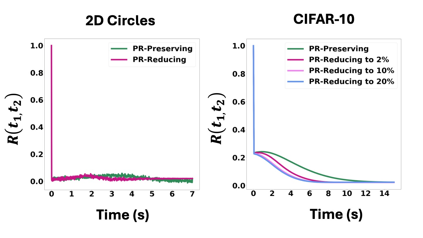
This is because, empirically, score estimates do not appear to be strongly auto-correlated in time (see plots of network residual auto-correlations (i.e., \( R(t_1, t_2) \)) below and Appendix C.3 for details), suggesting that \( \mathbf{\hat{s}}(\mathbf{x}, t) \), the score estimate, is well approximated as a scaled colored noise process and the corresponding pfODE as an SDE. In such a case, standard theorems for SDE integration show that while errors due to noise do accumulate, these can be mitigated by a careful choice of integrator and ultimately controlled by reducing step size (Kloeden & Platen, 1992; Mou et al., 2019).

Finally, we verified this empirically with both additional low-dimensional experiments (Additional Toy Calibration Experiments) and with round-trip integration of the pfODE in high-dimensional datasets (see Experiments on image benchmark datasets).